1. Bottleneck traffic congestion as a strategic situation

Road traffic congestion in cities is one of the major problems facing modern society. According to a document released in 2015 by the Road Bureau of the Ministry of Land, Infrastructure, Transport and Tourism, the annual time lost due to traffic congestion per person is about 40 hours, which is equivalent to 40% of the time spent in vehicles (about 100 hours). In addition to this enormous amount of wasted time, road traffic congestion also has caused adverse environmental effects such as noise, air pollution, and CO₂ emissions. National and local governments have invested a large amount of resources and have been working for many years to solve traffic congestion by expanding existing roads and constructing new roads. However, even if such efforts succeeded in temporarily relieving the traffic jams, the situation continues as a "cat and mouse" scenario in which the traffic jam occurs again with the passage of time.

Although there are various causes of traffic congestion, everyone is familiar with traffic congestion that occurs on roads with bottlenecks. As the name implies, a bottleneck is a narrow section of road similar to the mouth of a bottle, the shape of which hinders the smooth flow of traffic. Examples include bridges, tunnels, tollbooths, and road construction sites. A bottleneck has an upper limit on the number of vehicles that can pass through during a certain period of time, so traffic congestion will occur if too many drivers trying to pass through the bottleneck at the same time. In other words, the degree of congestion is determined by each driver's decision of when to pass through the bottleneck.

A strategic situation is one in which the benefits and results that one obtains depend not only on one's own actions, but also on the actions of others. We are surrounded with full of strategic situations other than traffic jams. The innumerable examples include games and sports that are a competition for victory or defeat, as well as price competitions, conflicts, resource acquisition competitions, auctions, and negotiations. In strategic situations, each person will choose their optimal behavior while considering the way in which others behave. Game theory is a tool for analyzing decision-making in such situations.

Research on applying game theory to bottleneck traffic congestion is gradually increasing. However, theoretical analysis alone cannot determine whether or not theoretical predictions deviate from actual human behavior, or how and why such deviation occurs. Ultimately, decisions are made by living human beings. Understanding the characteristics and patterns of human behavior through experiments will compensate for the shortcomings of existing research and will contribute to clarification of mechanisms for the occurrence and transition of congestion.

2. Problem of deciding departure times

A well-known model for analyzing bottleneck congestion is the single bottleneck model. This model was originally devised by Vickrey (1969), after which a basic model was developed by Arnott et al. (1990, 1993). Figure 1 shows the shape of the transportation network assumed by the model. There is one road from the residential area (O) to the central business district, or CBD (D), and there is one bottleneck on that road. All drivers want to arrive at the destination at a shared desired arrival time and use this road to commute to the CBD from the residential area. There is a limit to the number of vehicles that can pass through the bottleneck per unit of time, and it is impossible for all drivers to pass through at the same time (that is, it is not possible for all drivers to arrive at the CBD at the desired arrival time). Travel costs for commuting are represented by the following formula.

(Travel time cost due to waiting time and bottleneck transit time)
+
Early arrival cost or late arrival cost due to the difference between the actual arrival time and the desired arrival time)

Each driver selects their departure time so as to minimize their travel cost while predicting the departure time of other drivers.

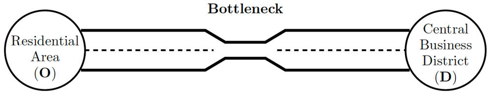Figure 1: Road with a single bottleneck

Here, I will introduce a numerical example with three drivers A, B, and C (hereinafter referred to as players). This example makes the following assumptions.

• Each player chooses the time of departing from the residential area to the CBD in a way which minimizes travel costs (the sum of travel time costs and early/late arrival costs).
• There are four departure times that each player can select: t = 0, 1, 2 and 3. The desired arrival time to the place of work is t = 2. This desired arrival time is common to all players.
• The travel time from the place of residence to the bottleneck entrance and the travel time from the bottleneck exit to the place of work shall both be 0. In other words, drivers arrive at the bottleneck at the same time as they depart from the residential area, and arrive at the CBD at the same time as they depart from the bottleneck.
• Only one driver can pass through the bottleneck per unit of time. If two or more players arrive at the bottleneck, the order of passing through the bottleneck is determined randomly.
• Travel time is calculated as follows: Time of arrival at the CBD - time of departure from the residential area. The travel time cost is 2 per unit of time.
• Early arrival time is calculated as follows: Desired arrival time - time of arrival at the CBD. The early arrival cost is 1 per unit of time.
• Late arrival time is calculated as follows: Time of arrival at the CBD - desired arrival time. The late arrival cost is 5 per unit of time.

Table 1 shows the results when player A departs from the residential area at t = 0, and players B and C depart from the residential area at t = 1. Player A passed without waiting at the bottleneck, but she arrived one unit of time earlier than the desired arrival time. Since players B and C departed at the same time, the first one to pass through the bottleneck was decided randomly. Player B passed through first and was able to arrive at the CBD at the desired time. Player C was kept waiting at the bottleneck entrance, and she was delayed by one unit of time from the desired arrival time.

Player	Departure time	Bottleneck		Arrival time	Early arrival time	Late arrival time	Travel cost
		Wait time	Pass through time
A	0	0	1	1	1	0	3
B	1	0	1	2	0	0	2
C	1	1	1	3	0	1	9

Table 1: Numerical example

In the case of analysis using game theory, we focus on a state known as the Nash equilibrium. The Nash equilibrium is a state in which each player's strategy (here, the departure time) best responds to the strategies of other players. In other words, this is a stable state in which nobody can get better off by unilaterally deviating to another strategy. If at least one player has an incentive to unilaterally deviate to another strategy, the state is not the Nash equilibrium.

The combination of departure times in Table 1 is not the Nash equilibrium. As a result, player C passed through the bottleneck after player B. However, since the order of passing through the bottleneck is randomly determined, player C's (expected) travel cost when choosing t = 1 is (2 + 9) / 2 = 5.5. Now, let's suppose that only player C changes the departure time to t = 0. Since this overlaps with player A's departure time, the order of passing through the bottleneck is randomly determined. If successfully passing through first without waiting, player C will arrive one unit of time earlier than the desired arrival time, so the travel cost will be 3 (travel time cost of 2 + early arrival cost of 1). If passing through the bottleneck after player A, player C will arrive at the place of work at her desired arrival time, although there is a waiting time of one unit of time. The travel cost in this case is 4 (travel time cost of 4 only). Therefore, player C's (expected) travel cost when choosing t = 0 is (3 +4) / 2 = 3.5. This means that player C's (expected) travel cost can be reduced compared to when the departure time is t = 1. This indicates that the combination of departure times in Table 1 is not the Nash equilibrium, as player C has an incentive to change her departure time from t = 1 to t = 0 if the other two players do not change their departure time.

The Nash equilibrium in this example occurs when all three players choose t = 0, and the total travel cost of the three players at that time is 18. In the combination of departure times in Table 1, the total travel cost of the three players is 14, which is lower than the total travel cost in the Nash equilibrium. If the minimum total travel cost of the three players is considered as the social optimum, it is clear that the combination of departure times of the Nash equilibrium does not achieve the social optimum. If one player were to depart at each time from t = 0 to t = 2, the total travel cost of the three players will be the minimum of 12, which is socially optimal. However, in this state, the travel cost is different for each player, and each player freely decides their own departure time without coordinating with the other players. Accordingly, it is very unlikely that the socially optimally state can spontaneously emerge.

3. How do actual people choose their departure time?

In the experiment I am going to run this year on the Tama Campus of Chuo University, about 10 to 20 students will be invited to each experiment session. A large number of players and strategies results in a large number of Nash equilibria, which requires numerical computations to derive them. Since all participants will face the same cost structure in the experiment, it is natural to consider a symmetric Nash equilibrium, an equilibrium in which all players adopt the same strategy, as a benchmark solution. For example, let's assume that there are 15 players and 21 departure times (t = 0, 1, 2, ..., 20) from which to choose, the desired arrival time is t = 15, and the travel time cost, early arrival cost, and late arrival cost per one unit of time are the same as in Table 1. In this case, each player will use the mixed strategy shown in Figure 2 (the top graph is a probability distribution, while the bottom graph is a cumulative distribution). This means that each player chooses the departure time according to the probability distribution in this figure. For example, the selection probability for t = 8 is 0.1581, the selection probability for t = 19 is 0.0090, and so on.

Now, which departure time would a real person choose if playing this game multiple times? Would each player's behavior conform to equilibrium play? Based on the enormous amount of experimental research performed thus far, I expect the following results.^[1] (1) The observed behavior on the aggregate level would be accounted well by the symmetric mixed-strategy Nash equilibrium; however, (2) there would be a wide variety of patterns of irrational behavior on the individual level, and only a few participants would behave in accordance with equilibrium play. In other words, I would observe heterogeneous patterns of behavior on the individual level coupled with systematic and replicable patterns of behavior on the aggregate level that seem to differ very little from equilibrium play.

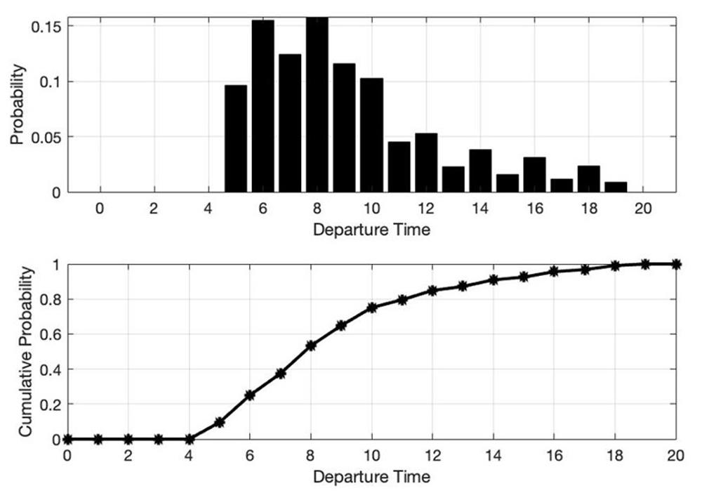
Figure 2: Symmetric mixed strategy Nash equilibrium

4. Initiatives for the future

There are several possible causes of deviations from the Nash equilibrium on the individual level. For example, game theory assumes perfectly rational players, but real people may rather be boundedly rational. Moreover, to begin with, people are commonly known to be heterogeneous, not homogeneous. Consequently, we may need to use an equilibrium concept that well captures variations in the individuality of players. One candidate is a model that incorporates the heterogeneity of players into the quantal response equilibrium that is capable of ascertaining bounded rationality. When looking ahead to data analysis after my experiment, I would like to proceed with the study of a game theory model that takes these two into consideration.

*This work was supported by JSPS KAKENHI Grant Number JP20K01554.

---

[1] A survey of experiments on the mixed strategy Nash equilibrium is detailed in Chapter 3 of Camerer (2003).

[Reference Literature]

Arnott, Richard, André de Palma, and Robin Lindsey. 1990. Economics of a bottleneck. Journal of Urban Economics 27: 111-130.
Arnott, Richard, André de Palma, and Robin Lindsey. 1993. A structural model of peak-period congestion: A traffic bottleneck with elastic demand. American Economic Review 83: 161-179.
Camerer, Colin. 2003. Behavioral Game Theory. Princeton University Press, New Jersey.
Vickrey, William S. 1969. Congestion theory and transport investment. American Economic Review 59: 251-260.

Hironori Otsubo／Associate Professor, Faculty of Global Management, Chuo University
Area of Specialization: Experimental Economics

Hironori Otsubo was born in Omuta City, Fukuoka Prefecture in 1976.
In May 2002, he graduated from the University of Arizona, USA.
In August 2008, he completed the Doctoral Program in the Graduate School of the University of Arizona, USA. He holds a Ph.D. in economics.
He served as a post-doctoral research associate at the Max Planck Institute of Economics in Germany and as a Full-time Lecturer/Associate Professor in the Faculty of Economics, Soka University before assuming his current position in April 2021.

• Share articles
• 
• 
•